The history says that in the latter half of the seventeenth century it was Galileo Galilei (Italian astronomer, physicist, engineer, philosopher, mathematician, 1564-1642) who noticed that the errors in the astronomical observations were not totally random. Instead, small and large errors were symmetrical distributed around a central value.
Then, during the first decade of the nineteenth century, two guys, Adrien-Marie Legendre (French mathematician, 1752-1833) and Carl Friedrich Gauss (German mathematician, 1777-1855), find out the precise mathematical formula, and Gauss demonstrated that this curve provided a close fit to the empirical distribution of observational errors. In fact, Gauss also derived the least squares method (statistical approach in regression analysis) from the assumption that the error were "normally" distributed.
Apart from physics applications, the normal distribution appeared in the mathematical field. It was Abraham de Moivre (French mathematician, 1667-1754) who showed that some binomial distributions could be approximated by one general curve. Actually, this general curve is the limiting case for a binomial distribution when the events have a 50/50 chance of happening and the trials go to infinity.
Let's take the example of the distribution of coin tosses. De Moivre saw that if the number of events started to increase, the shape of the binomial distribution approached a certain smooth curve. In this way, de Moivre immediately saw that if one can get the mathematical expression for this smooth curve, then it would be possible to find the probability of N heads out of M coin flips (where N<M, and both are large numbers). The curve is what we call now the "normal curve", and is expressed as follows:
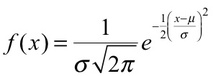
where "mu" (μ) is the mean or expectation of the distribution, and "sigma" (σ) is the standard deviation. The way to write the normal distribution was done by Karl Pearson (English mathematician and biostatistician, 1857-1936).
Many mathematicians were involved in building the concept of normal distribution, but it was Gauss who was more strongly linked. A direct consequence is that the term "Gaussian" is often used instead of "normal" or "bell-shape" curve. However, by the end of nineteenth century, some authors started to use the term "normal distribution" cause the distribution was seen as typical or common.
Nowadays, the normal distribution can be found in diverse fields and applications. From describing measurement error to, for example, describe the height/age distribution in biological species. The score of IQ tests is another example, since this score is based on positions in the normal distribution. Or the ground state of an quantum harmonic oscillator, and many other applications.
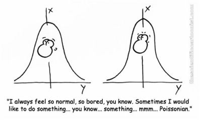
Even in this subject one can find some jokes about normal distribution, like:
Nowadays, the normal distribution can be found in diverse fields and applications. From describing measurement error to, for example, describe the height/age distribution in biological species. The score of IQ tests is another example, since this score is based on positions in the normal distribution. Or the ground state of an quantum harmonic oscillator, and many other applications.
Even in this subject one can find some jokes about normal distribution, like:
See you around!
Jesus
Jesus

 RSS Feed
